Quickstart Guide - OpenModelica

While using these models would require some familiarity with Modelica and OpenModelica, the packages have been setup so that users without such experience can run some basic simulations.

In the instructions below, we illustrate how to load the OpenIPSL library and the Example1 & Example2 packages and run a simulation for each of the packages.

Part 1: Installing OpenIPSL using OpenModelica’s Package Manager

• Download and install OpenModelica, here. The version used in this guide is 1.22.3.
• Follow the instructiosn in the following guide to add OpenIPSL into your OpenModelica installation and test that is working:
  • Slides: here
  • Video: here

Loading Example1 & Example2

1. Download the files of this repository by cloning with GIT. Alternatively, you can click here to download the *.zip file.
2. If you have cloned this repository, navigate to the location where it is stored. If you have downloaded the *.zip file, uncompress it in a directory to which you have read/write rights, e.g. C:\Users\myUserName\Documents\OM. You should now have a folder called CCTA-OpenIPSL-1.0.x.
3. Open OMEdit. If you can’t find it, look under C:\Program Files\OpenModelica1.22.3-64bit\bin and run OMEdit.exe by double-clicking.
4. Go to File > Open Model/Library Files(s) , and navigate the folder C:\Users\myUserName\Documents\OM\CCTA-OpenIPSL-1.0.1\CCTA-OpenIPSL-1.0.1\Example1, select the file package.mo and click on OMEdit’s Libraries browser: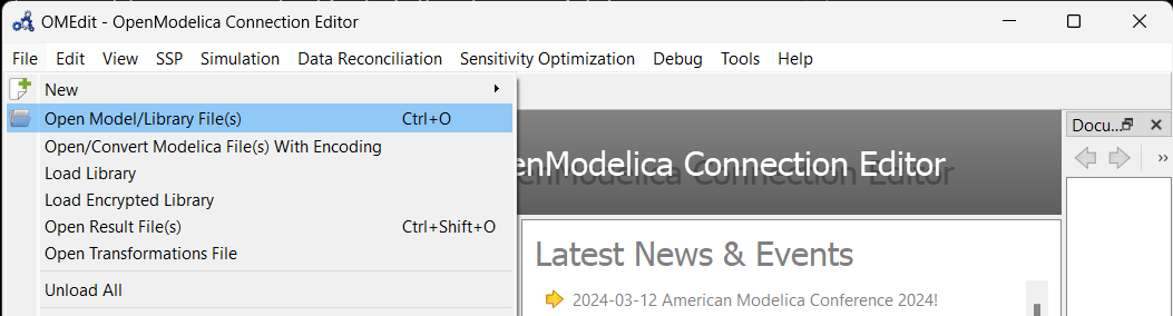 This will load Example1 and automatically load OpenIPSL (if if Part 1 has been completed) on Dymola’s Projects browser as shown below: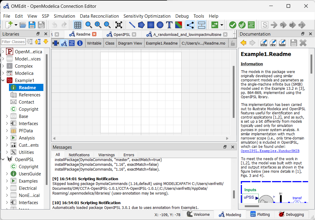 Note that OpenIPSL has been loaded automatically.
5. Repeat step 4, but instead, navigate to the sub-folder of Example 2, C:\Users\myUserName\Documents\OM\CCTA-OpenIPSL-1.0.1\CCTA-OpenIPSL-1.0.1\Example2, select the file package.mo and click on Open. This will load the package, Example2 in OMEdit Libraries browser as shown below.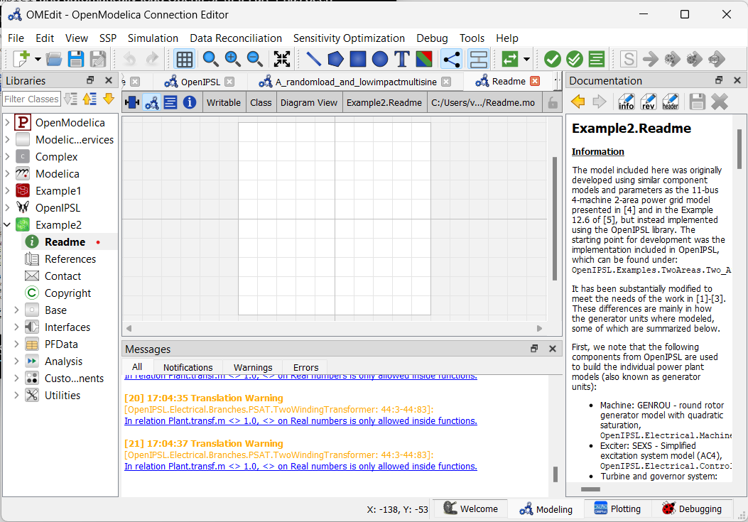

Sample Simulation

Simulating a model from Example1

1. In OMEdit’s Libraries browser, click through Example1 until reaching the example: Example1.Analysis.RedesignedControllerVerification.C0_8cycles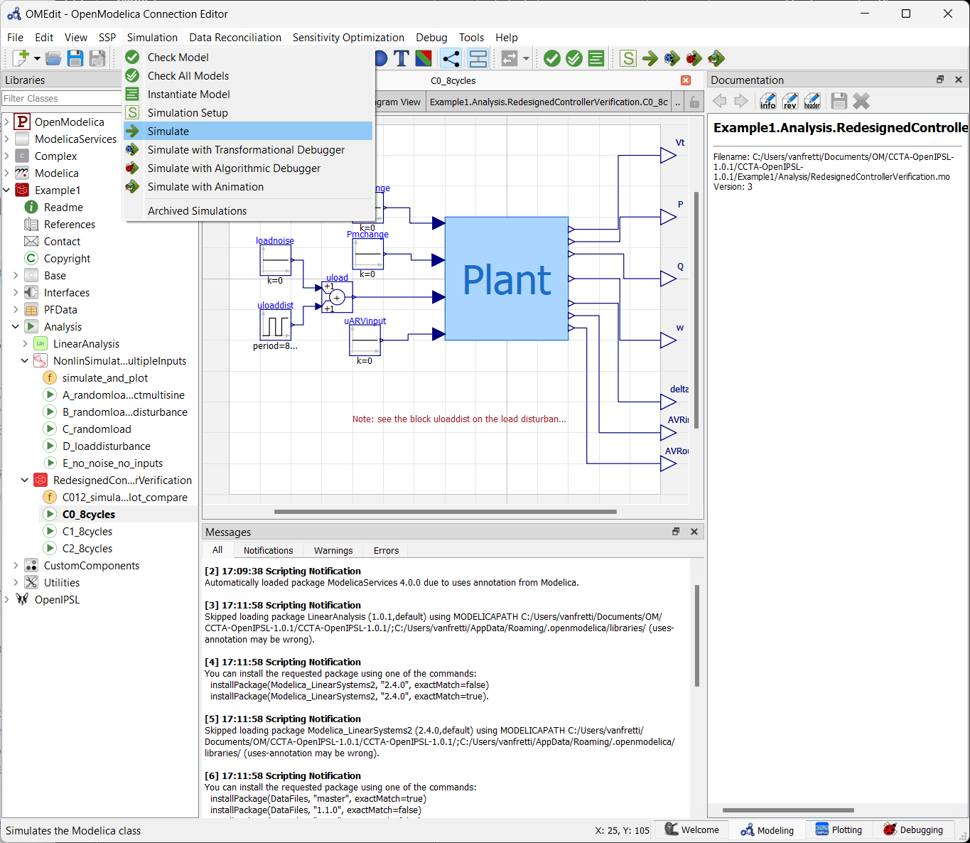
2. As shown in the the figure above, go to Simulation > Simulate, this will start the simulation, and the Plotting tab will appear.
3. When the simulation is completed, the Messages window will show at the bottom, The simulation finished successfully.
4. In the Variables window, select P to generate the plot displayed below, use the mouse to zoom in to reproduce the plot.
5. Repeat for any of the other sample simulation models, under Example1.Analysis.NonlinSimulationsMultipleInputs or Example1.Analysis.RedesignedControllerVerification.

   Simulating a model from Example2

   Similar to the models in Example1, several models are available in Example2 for simulation. As an example:

6. Navigate to Example2.Analysis.PFVariant.Ramping_pf, double click it and then go to Simulation Setup as shown in the figure below.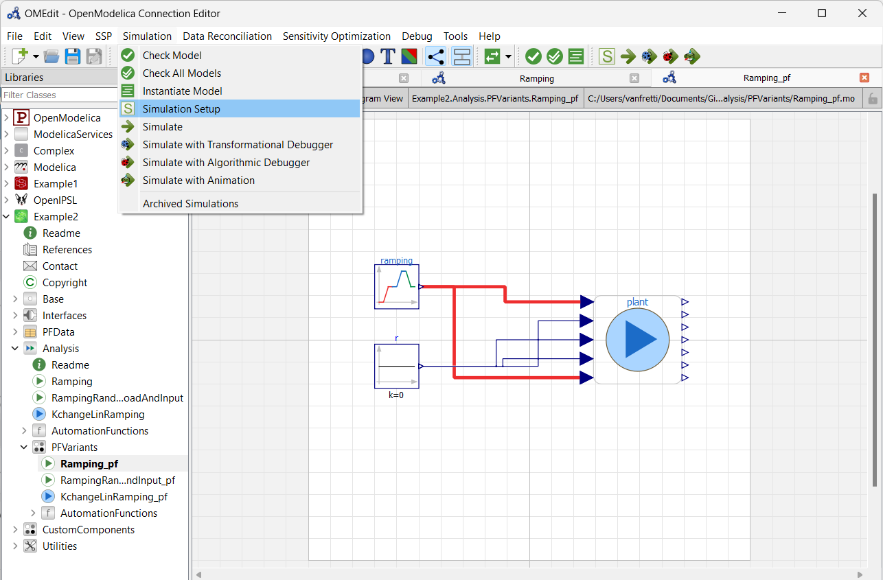
7. Configure the simulation setup as shown in the figure below. Make sure you set the the Stop Time to 300 sec and select only 1 in Number of Processors, then click on OK… get some :coffee: and relax, now you have to wait for the simulation to run!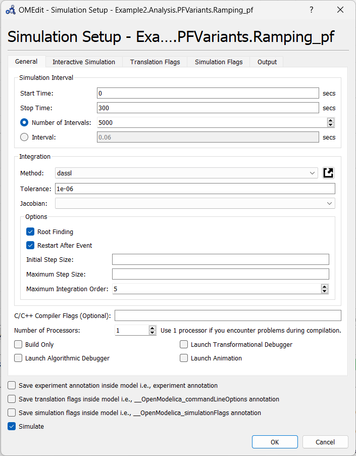
8. In the Plotting tab, go to the Variables window and select plant.P to reproduce the plot below.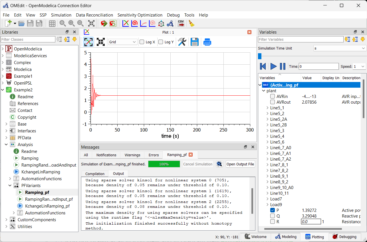

Important Note: OpenModelica has some challenges running the models in Example2 package. For example, the model above fails to simulate for longer time periods (e.g., set the Stop Time to 600 sec and see what happens!). To get an idea of the expected results, browse the documentation of the models in both Example1.Readme and Example2.Readme to get an idea of the expected output.

Automation via Scripting and Linear Analysis

Unfortunately it is not as straight forward to demonstrate how to automate simulation and linearization analysis as as in the case of using Dymola However, it is possible to automate simulations via scripting and perform linear analysis using the OMNotebook distributed with OpenModelica or using one of its interfaces, e.g. Python, MATLAB, etc. A tutorial on simulation automation analysis and linearization exxamples is provided in the tutorial that can be found here.

To go back to the main page, click here