Example1.Analysis.LinearAnalysis.CustomFunctions

Custom functions for automated analysis, including linearization and simulation, and their comparison

Information

This package contains two functions for automated analysis:

Simple linearization workflow: Example1.Analysis.LinearAnalysis.CustomFunctions.LinearizeSimple
Extended linearization workflow: Example1.Analysis.LinearAnalysis.CustomFunctions.LinearizeAndCompare

Extends from Modelica.Icons.FunctionsPackage (Icon for packages containing functions).

Package Content

Name	Description
LinearizeSimple	Linearize the model at any point in time tlin
LinearizeAndCompare	Linearize the model, simulate the linear model obtained and compare with the nonlinear model response.

Example1.Analysis.LinearAnalysis.CustomFunctions.LinearizeSimple

Linearize the model at any point in time tlin

Information

This function linearizes the non-linear model at any point in time specified by the user.

The results are displayed in the Commands Window.

The obtained linear model can be used in any other environment. The linear model is available in the file, dslin.mat, that will appear under your Dymola working directory. It can be loaded in MATLAB using the Dymola function:

[A,B,C,D,xName,uName,yName] = tloadlin('dslin.mat')

Add to the MATLAB workspace the directory and sub-directories under: C:\Program Files\Dymola 2024x\Mfiles

In addition, the file MyData.mat contains the y0 vector, which corresponds to the output vector at the point in time where linearization is performed.

Usage

In the Package Browser, right click on the function and select "Call function...". This will open the function's window.

Leave the default parameters on first use. Alternatively, modify the tlin and tsim parameters, note that tsim should be greater or equal to tlin.
Go to the bottom of the window and click on "Execute", if successful, messages/results are displayed in the command window.
Go back to the function's own window and click on "Close".

Sample Output

Executing the function gives the following results in the "Commands" window.

Example1.Analysis.LinearAnalysis.CustomFunctions.LinearizeSimple();

DAE Mode is turned off.

Global optimization is disabled.

Sparse options disabled.

Linearization and Nonlinear Model Comparison is starting...

Linearized Model

Number of states: 12

Simulating nonlinear model

= true

Redeclaring variable: Real y0 [7, 1012];

= true

Declaring variable: Real y0out [7];

y0 =

= "

y0 = =

1.000024318695068359375

0.196186602115631103515625

0.900009691715240478515625

1.28431034088134765625

2.50904435006304993294179e-07

2.120034694671630859375

[0.0, 376.9911183891212, 0.0, 0.0, 0.0, 0.0, 0.0, 0.0, 0.0, 0.0, 0.0, 0.0;

-0.17610876763748942, 0.0, 0.0, 0.0, -0.19586150145880193, 0.05515410219837237,

0.0, 0.0, 0.0, 0.0, 0.0, 0.0;

-0.25587785362300375, 0.0, -0.12499999997574654, 0.0, -0.2667630481888344,

-0.001159492170868593, 0.0, 0.0, 0.12499999999488744, 0.0, 0.0, 0.0;

0.4265899899207167, 0.0, 0.0, -1.0000000000939857, 0.007883244407403102,

-1.4901043751184482, 0.0, 0.0, 0.0, 0.0, 0.0, 0.0;

-3.3690289136967633, 0.0, 33.3333333351218, 0.0, -36.84568272027127,

-0.015266513308270566, 0.0, 0.0, 0.0, 0.0, 0.0, 0.0;

2.4254614215865864, 0.0, 0.0, 14.285714287056937, 0.04482173884230768,

-22.75799624545071, 0.0, 0.0, 0.0, 0.0, 0.0, 0.0;

-8.934890956417721, 0.0, 0.0, 0.0, 29.303251383490004, 33.12307890942945,

-66.66666667217629, 0.0, 0.0, 0.0, 0.0, 0.0;

0.0, 0.0, 0.0, 0.0, 0.0, 0.0, 0.0, -1.0, 0.0, 0.0, 0.0, 0.0;

0.0, 18999999.999786172, 0.0, 0.0, 0.0, 0.0, -2000000.0001652886,

10000.00082740371, -9999.999999590995, 0.0, 0.0, -18999999.99980534;

0.0, 0.009499999999893087, 0.0, 0.0, 0.0, 0.0, 0.0, 0.0, 0.0, -0.001, 0.0,

-0.009499999999902671;

0.0, 0.009499999999893087, 0.0, 0.0, 0.0, 0.0, 0.0, 0.0, 0.0, 0.0, -0.001,

-0.009499999999902671;

0.0, 0.7092198580776662, 0.0, 0.0, 0.0, 0.0, 0.0, 0.0, 0.0, 0.0, 0.0,

-0.7092198581570424],

[0.0, 0.0, 0.0, 0.0;

0.0, 0.14285715467719584, -0.03160725649463204, 0.0;

0.0, 0.0, -0.04042882695287631, 0.0;

0.0, 0.0, 0.10093337277083947, 0.0;

0.0, 0.0, -0.532308225276168, 0.0;

0.0, 0.0, 0.5738762639698587, 0.0;

0.0, 0.0, -1.0247506547026812, 0.0;

0.0, 0.0, 0.0, 0.0;

19000001.57206705, 0.0, 0.0, 2000000.1654807418;

0.009500000786033523, 0.0, 0.0, 0.0;

0.7092199168371426, 0.0, 0.0, 0.0],

[-0.13402336434626583, 0.0, 0.0, 0.0, 0.43954877075235005, 0.4968461836414418,

0.0, 0.0, 0.0, 0.0, 0.0, 0.0;

0.3043068141629995, 0.0, 0.0, 0.0, 1.4537261850177308, 0.7665888604391177, 0.0,

0.0, 0.0, 0.0, 0.0, 0.0;

1.2253264601006595, 0.0, 0.0, 0.0, 1.3643245623264468, -0.38254244268485077, 0.0,

0.0, 0.0, 0.0, 0.0, 0.0;

0.0, 0.9999999998895094, 0.0, 0.0, 0.0, 0.0, 0.0, 0.0, 0.0, 0.0, 0.0, 0.0;

1.0000000001010991, 0.0, 0.0, 0.0, 0.0, 0.0, 0.0, 0.0, 0.0, 0.0, 0.0, 0.0;

0.0, 9.499999999893086, 0.0, 0.0, 0.0, 0.0, 0.0, 0.0, 0.0, 0.0, 0.0,

-9.49999999990267;

0.0, 0.0, 0.0, 0.0, 0.0, 0.0, 0.0, 0.0, 0.9999999999590995, 0.0, 0.0, 0.0],

[0.0, 0.0, -0.015371259820540216, 0.0;

0.0, 0.0, 0.02120334463562301, 0.0;

0.0, 0.0, 0.21999579935538804, 0.0;

0.0, 0.0, 0.0, 0.0;

9.500000786033524, 0.0, 0.0, 1.0;

0.0, 0.0, 0.0, 0.0], {"uPSS", "uPm", "uPload", "uvsAVR"}, {"Vt", "Q", "P", "w",

"delta", "AVRin", "AVRout"}, {"Plant.G1.machine.delta", "Plant.G1.machine.w",

"Plant.G1.machine.e1q", "Plant.G1.machine.e1d", "Plant.G1.machine.e2q",

"Plant.G1.machine.e2d", "Plant.G1.avr.vm", "Plant.G1.avr.vr", "Plant.G1.avr.vf1",

"Plant.G1.pss.imLeadLag.TF.x_scaled[1]", "Plant.G1.pss.imLeadLag1.TF.x_scaled[1]",

"Plant.G1.pss.derivativeLag.TF.x_scaled[1]"}

Inputs

Name	Description
tlin	t for model linearization [s]
tsim	Simulation time [s]
pathToNonlinearPlantModel	Nonlinear model for linearization
pathToNonlinearExperiment	Nonlinear Model for simulation

Outputs

Name	Description
A[:, :]	A-matrix
B[:, :]	B-matrix
C[:, :]	C-matrix
D[:, :]	D-matrix
inputNames[:]	Modelica names of inputs
outputNames[:]	Modelica names of outputs
stateNames[:]	Modelica names of states

Example1.Analysis.LinearAnalysis.CustomFunctions.LinearizeAndCompare

Linearize the model, simulate the linear model obtained and compare with the nonlinear model response.

Information

This function can linearize the model at initialization or at a user provided point in time. Once the model is linearized, linear model and the nonlinear models are simulated.

The response of both models is then plotted/compared to check the quality of the linear model.

The function uses the following models:

Non-linear model for linearization: Example1.Analysis.LinearAnalysis.NonlinModel_for_Linearization
Non-linear model for simulation: Example1.Analysis.LinearAnalysis.NonlinModel_for_NonlinExperiment
Linear model for simualtion: Example1.Analysis.LinearAnalysis.LinearModelGeneral

After executing the function the results are displayed in the command window.

For post-processing, the follwing .mat files are generated with time simulation responses are produced:

res_lin.mat, containing the time response of the linear model obtained by linearizing the linear model for simulation.
res_nl.mat, containing the time response of the non-linear model.
res_nl_beforedist.mat, containing the time response of the non-linear model up to the poin in time where the model is linearized. This is used to extract the y0 output vector that is used in the linear model for simulation.
These files can be opened in MATLAB using the dymbrowse tool. Add to the MATLAB workspace the directory and sub-directories under: C:\Program Files\Dymola 2024x\Mfiles, and in the command window of MATLAB enter: dymbrowse and selected the data to plot.

The linearized model is contained in the following .mat files:

MyData.mat contains the y0 vector, which corresponds to the output vector at the point in time where linearization is performed.
dslin.mat contains the linear model obtained at the specified point for lineariation.
The obtained linear model can be used in any other environment. The linear model is available in the file, dslin.mat. It can be loaded in MATLAB using the Dymola function [A,B,C,D,xName,uName,yName] = tloadlin('dslin.mat')

Usage

In the Package Browser, right click on the function and select "Call function...". This will open the function's window.

Leave the default parameters on first use. Alternatively, modify the tlin and tsim parameters, note that tsim should be greater or equal to tlin.
Go to the bottom of the window and click on "Execute", if successful, messages/results are displayed in the command window.
Go back to the function's own window and click on "Close".

Sample Output

Executing the function gives the following plot is produced in the "Simulation" window and the following results in the "Commands" window.

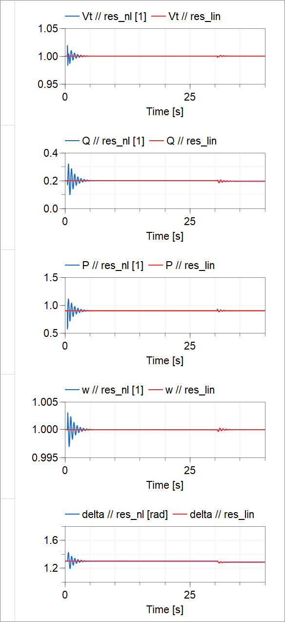
Example1.Analysis.LinearAnalysis.CustomFunctions.LinearizeAndCompare();

DAE Mode is turned off.

Global optimization is disabled.

Sparse options disabled.

Linearization and Nonlinear Model Comparison is starting...

= true

Simulating nonlinear model

= true

y0 before disturbance =

= "

0.998271

0.203063

0.921617

1.29897

-3.55698e-11

2.12495

Simulating linear model

= true

= 1

[0.0, 376.99111838906373, 0.0, 0.0, 0.0, 0.0, 0.0, 0.0, 0.0, 0.0, 0.0, 0.0;

-0.17610876767279915, 0.0, 0.0, 0.0, -0.19586150142483613, 0.05515410219997556,

0.0, 0.0, 0.0, 0.0, 0.0, 0.0;

-0.25587785359503384, 0.0, -0.12500000002903436, 0.0, -0.2667630481021101,

-0.001159492170902296, 0.0, 0.0, 0.12500000001466172, 0.0, 0.0, 0.0;

0.42658999050935953, 0.0, 0.0, -0.9999999998908723, 0.007883244274318683,

-1.4901043751617613, 0.0, 0.0, 0.0, 0.0, 0.0, 0.0;

-3.369028913176898, 0.0, 33.33333333281978, 0.0, -36.84568271688989,

-0.015266512953637873, 0.0, 0.0, 0.0, 0.0, 0.0, 0.0;

2.425461424825778, 0.0, 0.0, 14.285714284155317, 0.0448217383657263,

-22.75799624611222, 0.0, 0.0, 0.0, 0.0, 0.0, 0.0;

-8.934890939628422, 0.0, 0.0, 0.0, 29.303251372407868, 33.1230788990298,

-66.66666667021094, 0.0, 0.0, 0.0, 0.0, 0.0;

0.0, 0.0, 0.0, 0.0, 0.0, 0.0, 0.0, -1.0, 0.0, 0.0, 0.0, 0.0;

0.0, 18999999.999783278, 0.0, 0.0, 0.0, 0.0, -2000000.0001063284,

10000.00082740371, -10000.000001172937, 0.0, 0.0, -18999999.996308953;

0.0, 0.00949999999989164, 0.0, 0.0, 0.0, 0.0, 0.0, 0.0, 0.0, -0.001, 0.0,

-0.009499999998154478;

0.0, 0.00949999999989164, 0.0, 0.0, 0.0, 0.0, 0.0, 0.0, 0.0, 0.0, -0.001,

-0.009499999998154478;

0.0, 0.7092198580775582, 0.0, 0.0, 0.0, 0.0, 0.0, 0.0, 0.0, 0.0, 0.0,

-0.7092198580803518],

[0.0, 0.0, 0.0, 0.0;

0.0, 0.14285715467719584, -0.03160719305331635, 0.0;

0.0, 0.0, -0.040428715930573844, 0.0;

0.0, 0.0, 0.10093331725968824, 0.0;

0.0, 0.0, -0.5323070687938507, 0.0;

0.0, 0.0, 0.5738766604780818, 0.0;

0.0, 0.0, -1.024765457676343, 0.0;

0.0, 0.0, 0.0, 0.0;

19000001.57206705, 0.0, 0.0, 2000000.1654807418;

0.009500000786033523, 0.0, 0.0, 0.0;

0.7092199168371426, 0.0, 0.0, 0.0],

[-0.1340233640944263, 0.0, 0.0, 0.0, 0.43954877058611797, 0.496846183485447, 0.0,

0.0, 0.0, 0.0, 0.0, 0.0;

0.3043068137697762, 0.0, 0.0, 0.0, 1.4537261847736198, 0.7665888603335728, 0.0,

0.0, 0.0, 0.0, 0.0, 0.0;

1.2253264605206322, 0.0, 0.0, 0.0, 1.364324561691764, -0.38254244286640693, 0.0,

0.0, 0.0, 0.0, 0.0, 0.0;

0.0, 0.9999999998893571, 0.0, 0.0, 0.0, 0.0, 0.0, 0.0, 0.0, 0.0, 0.0, 0.0;

1.0000000001610603, 0.0, 0.0, 0.0, 0.0, 0.0, 0.0, 0.0, 0.0, 0.0, 0.0, 0.0;

0.0, 9.499999999891639, 0.0, 0.0, 0.0, 0.0, 0.0, 0.0, 0.0, 0.0, 0.0,

-9.499999998154477;

0.0, 0.0, 0.0, 0.0, 0.0, 0.0, 0.0, 0.0, 1.0000000001172937, 0.0, 0.0, 0.0],

[0.0, 0.0, -0.01537148186514514, 0.0;

0.0, 0.0, 0.02120284503526193, 0.0;

0.0, 0.0, 0.21999546628848066, 0.0;

0.0, 0.0, 0.0, 0.0;

9.500000786033524, 0.0, 0.0, 1.0;

0.0, 0.0, 0.0, 0.0], {"uPSS", "uPm", "uPload", "uvsAVR"}, {"Vt", "Q", "P", "w",

"delta", "AVRin", "AVRout"}, {"Plant.G1.machine.delta", "Plant.G1.machine.w",

"Plant.G1.machine.e1q", "Plant.G1.machine.e1d", "Plant.G1.machine.e2q",

"Plant.G1.machine.e2d", "Plant.G1.avr.vm", "Plant.G1.avr.vr", "Plant.G1.avr.vf1",

"Plant.G1.pss.imLeadLag.TF.x_scaled[1]", "Plant.G1.pss.imLeadLag1.TF.x_scaled[1]",

"Plant.G1.pss.derivativeLag.TF.x_scaled[1]"}, {0.9982708096504211,

0.20306333899497986, 0.9216165542602539, 1.0, 1.2989709377288818,

-3.5569769352150615E-11, 2.124945878982544}

Inputs

Name	Description
tlin	t for model linearization [s]
tsim	Simulation time [s]
numberOfIntervalsin	No. of intervals
methodin	Solver
fixedstepsizein	Time step - needed only for fixed time step solvers
pathToNonlinearPlantModel	Nonlinear plant model
pathToNonlinearExperiment	Nonlinear experiment model
pathToLinearExperiment	Linear model for simulation

Outputs

Name	Description
A[:, :]	A-matrix
B[:, :]	B-matrix
C[:, :]	C-matrix
D[:, :]	D-matrix
inputNames[:]	Modelica names of inputs
outputNames[:]	Modelica names of outputs
stateNames[:]	Modelica names of states
y0out[:]	Initial value of the output variables

Automatically generated Wed Mar 13 11:30:38 2024.