Example2.Analysis.AutomationFunctions

Provides functions for automation of simulation and linearization using the models of the upper layer package

Information

This package contains functions that automate the simulation, plotting and linearization of the models under Example2.Analysis.

Extends from Modelica.Icons.FunctionsPackage (Icon for packages containing functions).

Package Content

Name	Description
simulate_and_plot_ramping	Simulates and plots the "Ramping" model
simulate_and_plot_inputs	Simulates and plots the "RampingRandomLoadAndInput" model to reproduce the results in Fig. 4 of [2].
linearize_KchangeLinRamping	Function to linearize the model KchangeLinRamping at any point in time.

Example2.Analysis.AutomationFunctions.simulate_and_plot_ramping

Simulates and plots the "Ramping" model

Information

Usage:

1. In the Package Browser, right click on the function and select "Call function...". This will open the function's window.



2. In the new function window, click on "Execute", if successful, messages/results are displayed in the command window and plots will appear in Simulation tab.
3. Go back to the function's own window and click on "Close".

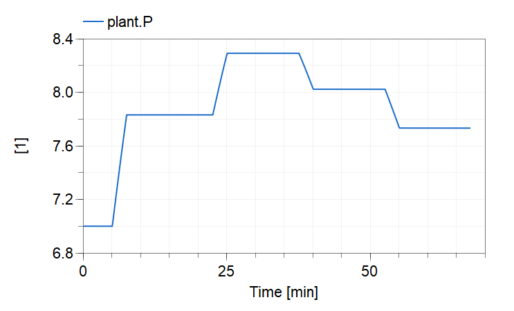
Sample Output:

Running the function will result in the following plot.

Extends from Modelica.Icons.Function (Icon for functions).

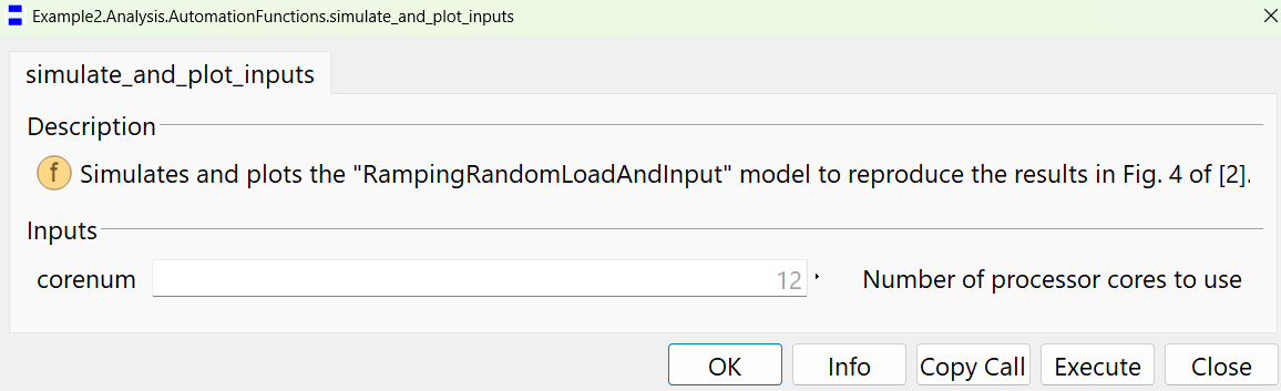
Example2.Analysis.AutomationFunctions.simulate_and_plot_inputs

Simulates and plots the "RampingRandomLoadAndInput" model to reproduce the results in Fig. 4 of [2].

Information

Usage:

1. In the Package Browser, right click on the function and select "Call function...". This will open the function's window.



2. Enter the desired number of cores to use in "corenum". The number of cores to use depends on your computer's resources. , if your computer has more than 12 cores, you can enter the desired number of cores to use in the function's main window. Note that it will take some trial an error to find a trade off on the number of cores to use in your system as per Amdahl's law. See the note below the sample output for more details.
3. In the new function window, click on "Execute", if successful, messages/results are displayed in the command window and plots will appear in Simulation tab.
4. Go back to the function's own window and click on "Close".

Sample output:

Running the function will result in the following plot.

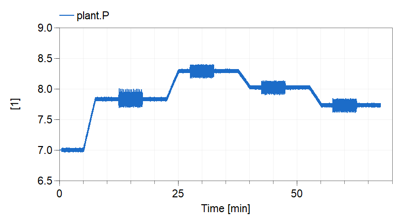
Note:

Please observe that running this function involves simulating the Example2.Analysis.RampingRandomLoadAndInput model, which takes subtantially more time compared to example Example2.Analysis.Ramping, the reason is that both random load and probing signals are added to the model which results in an additional computation burden.

This function calls the Example2.Utilities.SetupSolverSettings.On function that configures several flags to improve simulation speed, however, even by enabling these features, the simulation is time consuming.

For example, running the model using a computer with an 13th Gen Intel(R) Core(TM) i9-13900K, 3.00 GHz, processor and 128 GB DDR4 RAM, setup to use 12 cores, gave the following metrics:

Integration terminated successfully at T = 4050

CPU-time for integration : 1.14e+03 seconds

CPU-time for one grid interval : 227 milliseconds

CPU-time for initialization : 0.004 seconds

Number of result points : 961436

Number of grid points : 5001

Number of accepted steps : 9072834

Number of f-evaluations (dynamics) : 18084763

Number of crossing function evaluations : 9575493

Number of Jacobian-evaluations : 3918760

Number of model time events : 476996

Number of input time events : 0

Number of state events : 3815

Number of step events : 0

Minimum integration stepsize : 2.78e-10

Maximum integration stepsize : 0.00922

Maximum integration order : 5

Looking at the first two lines of the metrics shows that running the model for 67.5 min (4050 sec.) took 19 min (1.14e+03 sec.).

Naturally, using a computer with a weaker processor and lower memory will lead to longer run times.

Recall that the purpose of this simulation is to use it as input for system identification purposes as explained in [2]. If this is not necessary for your purposes, it is recommended that you run instead the function Example2.Analysis.AutomationFunctions.simulate_and_plot_ramping, which takes substantially less time to execute.

Extends from Modelica.Icons.Function (Icon for functions).

Inputs

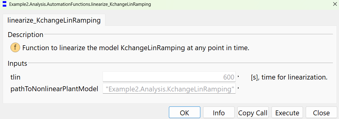
Example2.Analysis.AutomationFunctions.linearize_KchangeLinRamping

Function to linearize the model KchangeLinRamping at any point in time.

Information

Usage:

1. In the Package Browser, right click on the function and select "Call function...". This will open the function's window.



2. Enter the time for linearization, Example2.Analysis.KchangeLinRamping will be simulated until that point in time and linearized.
3. In the new function window, click on "Execute", if successful, messages/results are displayed in the command window and plots will appear in Simulation tab.
4. Go back to the function's own window and click on "Close".

Sample Output:

Executing the function will produce the following output in the "Commands" window.

Example2.Analysis.AutomationFunctions.linearize_KchangeLinRamping();

Setting up things...

DAE Mode is turned off.

Global optimization is disabled.

Sparse options disabled.

Number of cores reset to default:1

Starting simulation and linearization...

Declaring Modelica_LinearSystems2.StateSpace ss 

System not printed since too large (only dimensions):

   ss.A[52,52]

   ss.B[52,2]

   ss.C[1,52]

   ss.D[1,2]

The linear model is in your working directory.

Open the dslin.mat file following the instructions in the documentation.

You can also analyze the linear model using Dymola, for example typing in the commands window

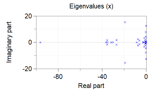
  Modelica_LinearSystems2.StateSpace.Plot.polesAndZeros(ss, zeros=false, print=true);

  will give you the polte plot shown in the Simulation tab and printed below.

Eigenvalues

The following pole plot is generated in the Simulation tab:

Post-processing in MATLAB:

The obtained linear model can be used in any other environment. The linear model is available in the file, dslin.mat, that will appear under your Dymola working directory. It can be loaded in MATLAB using the function:

[A,B,C,D,xName,uName,yName] = tloadlin('dslin.mat')

To use this function, add to the MATLAB workspace the directory and sub-directories under: C:\Program Files\Dymola 2024x\Mfiles

Extends from Modelica.Icons.Function (Icon for functions).

Inputs